Kibana Advanced Vega
Vega* is a Kibana visualization used to design complex, highly-customizable interactive visualizations. In this section we will start from scratch and go through a complete example in order to highlight the principal features and how to implement them.
Vega Paradigm
To configure a visualization, Vega has a few important keywords that let you transform your data and map from raw information to graphical elements.
{
  "$schema": "https://vega.github.io/schema/vega/v3.json",
  "width": 900,
  "height": 560,
  "padding": {"top": 0, "left": 0, "right": 0, "bottom": 0},
  "signals": [],
  "data": [],
  "scales": [],
  "marks": []
}
- signal : set variables that may react to user 's input
- data : load and transform datasets
- scales : scale your data (usually for plotting purposes)
- marks : define graphical elements plotted on the screen
width, height and padding are default signals used to set the dimension of your visualization.
Use case description
The Data we use is a collection of connections between two IP . For each IP we also know the country it came from. We want to plot the interactions between these IP on a single graph that allows to understand quickly how frequently two IP exchange packets and which countries are involved in these exchanges.
A single data looks like :
{
  "ip_source": "10.10.0.1",
  "ip_destination": "10.10.0.3",
  "country_source": "France",
  "country_dest": "Italie"
}
For the sake of simplicity, we are going to start using a static dataset of a very few connections. Further we are going to see how to extract the data directly from an Elasticsearch index.
Let 's get started.
Load the data
A Vega visualization is configured in JSON format. There are a few important keywords used to define how to configure your visualization. The first one is data which loads and transforms datasets.
Open a new Online Vega Editor and add an entry data object in which we define our static dataset :
{
  "$schema": "https://vega.github.io/schema/vega/v3.json",
  "width": 900,
  "height": 560,
  "padding": {"top": 0, "left": 0, "right": 0, "bottom": 0},
  "signals": [],
  "data": [
    {
      "name": "connections",
      "values": [
        {
          "ip_source": "10.10.0.1",
          "ip_destination": "10.10.0.3",
          "country_source": "France",
          "country_dest": "Italie"
        },
        {
          "ip_source": "10.10.0.1",
          "ip_destination": "10.10.0.2",
          "country_source": "France",
          "country_dest": "France"
        },
        {
          "ip_source": "10.10.0.4",
          "ip_destination": "10.10.0.2",
          "country_source": "Italie",
          "country_dest": "France"
        },
        {
          "ip_source": "10.10.0.3",
          "ip_destination": "10.10.0.1",
          "country_source": "Italie",
          "country_dest": "France"
        },
        {
          "ip_source": "10.10.0.4",
          "ip_destination": "10.10.0.5",
          "country_source": "Italie",
          "country_dest": "Maroc"
        },
        {
          "ip_source": "10.10.0.4",
          "ip_destination": "10.10.0.5",
          "country_source": "Italie",
          "country_dest": "Maroc"
        }
      ]
    }
  ],
  "scales": [],
  "marks": []
 }
VEGA provides useful commands to understand how your data is formatted.
Open the developer console (Ctrl+Maj+I on Firefox) and type
VEGA_DEBUG.view.data("connections").
Format the data
To plot our graph, we need to explicit exactly which IP are present in our DataSet. To do so, we define a new data set based on [connections] that we are going to transform. Add this code as a new data entry :
{
      "name": "IPs",
      "source": ["connections"],
      "transform": [
        {"type": "fold", "fields": ["ip_source", "ip_destination"], "as": ["key", "IP"]},
        {"type": "aggregate", "groupby": ["IP"]},
        {"type": "project", "fields": ["IP"]}
      ]
}
We use 3 different transformations to go from connections to the dataset we wanted.
- fold : extract every IP contained in ip _source or ip _dest and store it in a field IP.
- aggregate, groupby IP : group our Dataset according to their IP field and count how many occurrences of each IP is seen.
- project : filter the fields in we are interested in.
Note
Remember that you can take a look at our IPs dataSet by
typing VEGA_DEBUG.view.data("IPs")
Notice that we lost the country in the process. Let's add a few transformations :
- formula : The formula transform extends data objects with new values according to a calculation formula written in a subset of JavaScript. Refer to Vega documentation for more information.
- collect : collect all the objects in a data stream within a single array, allowing to sort by country values
{
   "name": "IPs",
   "source": ["connections"],
   "transform": [
        {"type": "fold", "fields": ["ip_source", "ip_destination"], "as": ["key", "IP"]},
        {"type": "formula", "expr": "datum.key == 'ip_source' ? datum.country_source : datum.country_dest", "as": "country"},
        {"type": "aggregate", "groupby": ["IP", "country"]},
        {"type": "project", "fields": ["IP", "country"]},
        {"type": "collect", "sort": {"field": "country"}}
    ]
}
Note
In VEGA, the keyword « datum » is reserved and references the current data.
Define plot variables
We want to plot our IP on a circle so we need to clarify for each IP its exact position on our visualization. Let's first define a variable for the radius of our circle. In Vega, a variable is signal object. Signals are dynamic variables that may react to user's input. For our purpose, a constant signal name will be sufficient. Add a new signal to our entry signals.
{"name": "radius", "value": 200}
Let's define the geometry of our plot. We need to define for each IP object his position on our visualization and some information related to how it should be plotted. Add these transformations to the IPs transforms argument :
        {"type": "window", "ops": ["cume_dist"], "as": ["order"]},
        {"type": "formula", "expr": "datum.order * 2 * PI", "as": "angle"},
        {"type": "formula", "expr": "inrange(datum.angle, [PI/2, 3*PI/2])", "as": "leftside"},
        {"type": "formula", "expr": "width/2 + radius * cos(datum.angle)", "as": "x"},
        {"type": "formula", "expr": "height/2 + radius * sin(datum.angle)", "as": "y"}
Let 's plot !
The keyword marks is used to define the elements plotted on the screen. Each mark defines a graphical element. We are going to define a first mark that represents our IPs in circle.
As you may notice, the angle attribute is defined in radian but an angle in degree is required. With Vega you can easily do these kind of conversion using the keyword scales. This is an elegant way to map from your data to visual elements.
Let's define a scale for our conversion :
{
     "name": "toDegree",
     "domain": [0,6.283185],
     "range": [0,360]
}
We can now add a mark for our plot. Notice that it used the scales that we just defined.
    {
      "type": "text",
      "name": "plotIP",
      "from": {"data": "IPs"},
      "encode": {
        "enter": {
          "text": {"field": "IP"},
          "x": {"field": "x"},
          "dx": {"signal": "datum.leftside ? -radius*0.05: radius*0.05"},
          "y": {"field": "y"},
          "angle": {"scale" : "toDegree", "signal": "datum.leftside ? datum.angle + PI : datum.angle"},
          "align": {"signal": "datum.leftside ? 'right' : 'left'"}
        }
      }
    }
You should see our IPs plotted in circle. We can add a mark element to plot a circle if we want to. Try to add the following to your mark attribute :
    {
      "type": "symbol",
      "encode": {
        "enter": {
          "fill": {"value": "#ccc"},
          "stroke": {"value": "#652c90"},
          "x": {"signal": "width/2"},
          "y": {"signal": "height/2"},
          "size": {"signal": "3.14159*radius*radius*1.2732"},
          "shape": {"value": "circle"},
          "opacity": {"value": 0.2},
          "strokeWidth": {"value": 5}
        }
      }
    }
Let's now plot our paths. First we need to create a dataset that contains all the information needed to plot the paths correctly (in the data entry) :
 {
  "name": "plotConnections",
  "source": "connections",
  "transform": [
    {"type": "aggregate", "groupby": ["ip_destination", "ip_source"]},
    {"type": "lookup", "from": "IPs", "key": "IP", "fields": ["ip_source"], "values": ["x", "y"], "as": ["x_source","y_source"]},
    {"type": "lookup", "from": "IPs", "key": "IP", "fields": ["ip_destination"], "values": ["x", "y"], "as": ["x_destination", "y_destination"]},
    {"type": "linkpath", "sourceX": {"expr": "datum.x_source"}, "targetX": {"expr": "datum.x_destination"}, "sourceY": {"expr": "datum.y_source"}, "targetY": {"expr": "datum.y_destination"}, "shape": "diagonal"}
  ]
 }
We also define the mark that uses this dataset to create our paths :
         {
          "type": "path",
          "from": {"data": "plotConnections"},
          "encode": {
            "enter": {
              "stroke": [{"value": "black"}],
              "strokeOpacity": [{"value": 0.8}],
              "strokeWidth": {"signal": "max(min(sqrt(datum.count), 15),1)"},
              "strokeCap": {"value": "round"},
              "strokeDash": {"value": [10, 10]},
              "x": {"value": 0},
              "y": {"value": 0},
              "path": {"field": "path"}
            }
          }
         }
You just saw the basics on how to create a graph with Vega. You first need to define the dataset (data entry) used for the different plots, using transformations if necessary. Then you need to precise the graphical elements you want Vega to plot on your visualization using the mark entry. scales can be used to map from data to visual elements. signals is used to define variables.
Get your data from elasticsearch
Getting you data from Elasticsearch is pretty straightforward if you know how to express your query. Our example was initially designed to be used on the Punchplatform livedemo. Open a new Vega visualization and insert your code. We are going to make a new dataset connections that loads the data directly from Elasticsearch.
We want to get the data from the mytenant-events- * index. In our case, our Elasticsearch query looks like :
GET online-mytenant-events-*/_search
{
 "_source": ["init.usr.loc.country", "target.host.ip", "channel"],
 "query": {
   "bool": {
     "filter": [
     {
       "exists": {"field": "init.usr.loc.country"}
     },
     {
       "term": {"channel": "ufw"}
     }
     ]
   }
 }
}
To create the associated dataset, you just need to set a few parameters and insert the query in the [body] argument. The dataset that uses this query looks like:
    {
      "name": "connections",
      "url": {
        "index": "mytenant-events-*",
        "body": {
          "_source": [
            "init.host.ip",
            "target.host.ip",
            "init.usr.loc.country",
            "target.usr.loc.country"
          ],
          "query": {
            "bool": {
              "filter": [
                {
                  "exists": {
                    "field": "init.usr.loc.country"
                  }
                },
                {
                  "term": {
                    "channel": "ufw"
                  }
                }
              ]
            }
          }
        },
        "size": 400
      },
      "format": {
        "property": "hits.hits"
      },
      "transform": [
        {
          "type": "project",
          "fields": [
            "_source.target.host.ip",
            "_source.init.host.ip",
            "_source.init.usr.loc.country",
            "_source.target.usr.loc.country"
          ],
          "as": [
            "ip_destination",
            "ip_source",
            "country_source",
            "country_dest"
          ]
        }
      ]
    }
Notice that we use a transformation to rename the variable and make this dataset compatible with our example.
Going further : Sort IPs by countries
To visualize more information, we can regroup IP by countries to see the countries involved in the exchanges. To do so we are going to plot an arc of circle for each IP with a color that defines the country.
If we want to plot these arcs of circle, we need to know exactly how many elements are present in our IPs dataset (the length of the arc is a fraction of the number of elements). To do so let 's add to new transformations to our ÌPs dataset :
{"type": "identifier", "as": "id"},
{"type": "extent", "field": "id", "signal": "minmaxID"}
- identifier : assign a unique id to each element
- extent : create a signal from a dataset
By doing so we create a signal minmaxID that contains the range of value of id that we just created.
If we want to assign a color to each country we need to create a scale object that maps from countries to colors.
{
  "name": "colorcountry",
  "type": "ordinal",
  "domain": {"data": "IPs", "field": "country"},
  "range": {"scheme": "category20"}
}
We now have enough information to plot these arcs of circle. Add a new mark object :
{
 "type": "arc",
 "name": "viewCountry",
 "from": {"data": "IPs"},
 "encode": {
   "enter": {
     "startAngle": {"signal": "(datum.angle)+PI/2 -PI/ minmaxID[1] "},
     "endAngle": {"signal": "datum.angle+PI/2 +PI/ minmaxID[1]"},
     "outerRadius": {"signal": "radius*1.04"},
     "innerRadius": {"signal": "radius"},
     "x": {"signal": "width/2"},
     "y": {"signal": "height/2"},
     "opacity": {"value": 1},
     "fill": {"scale": "colorcountry", "field": "country"}
    }
  }
}
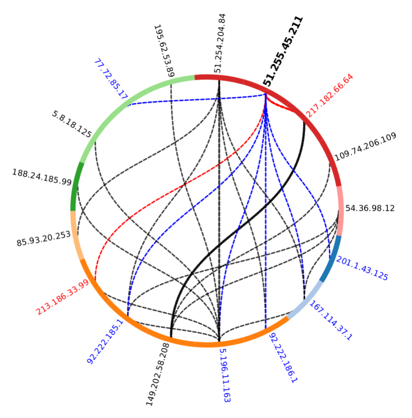
Going further : Add cursor interactions
With Vega you can add a lot a graphical interactions to visualize your data. In our example, we are interested in highlighting the connections that involve one precise IP while our cursor is mousing over this IP.
First, we need to know on which IP the cursor is. To do so, we use a signal named that updates whenever the cursor is on an IP element.
 {
  "name": "active",
  "value": null,
  "on": [
    {"events": "@plotIP:mouseover", "update": "datum.IP"},
    {"events": "mouseover[!event.item]", "update": "null"}
  ]
 }
Note
To ensure that everything is working properly, try to visualize the signal while your cursor is on an IP by typing ``VEGA_DEBUG.view.signal("active")
We need to know which IP exchanged with the [active] IP. To do so we create a dataset that contains only the connections in which either the active IP is a source or a destination :
{
 "name": "selected",
 "source": "connections",
 "transform": [{"type": "filter", "expr": "datum.ip_destination === active || datum.ip_source === active"}]
}
If you look at our plotIP mark, you may notice that all the description is encapsulated in the enter field. This field is used when you want Vega to interpret the content only once, when the visualization is first instantiated. If you want a mark to be reactive, you need to precise your argument in an update field. Our plotIP mark become :
    {
      "type": "text",
      "name": "plotIP",
      "from": {"data": "IPs"},
      "encode": {
        "enter": {
          "text": {"field": "IP"},
          "x": {"field": "x"},
          "dx": {"signal": "datum.leftside ? -radius*0.05: radius*0.05"},
          "y": {"field": "y"},
          "angle": {"scale": "toDegree", "signal": "datum.leftside ? datum.angle + PI : datum.angle"},
          "align": {"signal": "datum.leftside ? 'right' : 'left'"}
        },
        "update": {
          "fontSize": [{"test": "datum.IP === active", "value": 15}, {"value": 12}],
          "fontWeight": [{"test": "datum.IP === active", "value": "bold"}, {"value": "normal"}],
          "fill": [
            {"test": "datum.IP === active", "value": "black"},
            {"test": "indata('selected', 'ip_source', datum.IP)", "value": "blue"},
            {"test": "indata('selected', 'ip_destination', datum.IP)", "value": "red"},
            {"value": "black"}
          ]
        }
      }
    }
Let 's add a similar interaction to our path dataset, in an update field :
        {
          "stroke": [
            {"test": "datum.ip_destination === active", "value": "blue"},
            {"test": "datum.ip_source === active", "value": "red"},
            {"value": "black"}
          ],
          "strokeOpacity": [
            {"test": "(datum.ip_destination === active | datum.ip_source === active)", "value": 1},
            {"value": 0.8}
          ]
        }
Full code
You can copy paste this code into your Vega online editor to see the visualisation on the sample dataset
{
  "$schema": "https://vega.github.io/schema/vega/v3.json",
  "width": 900,
  "height": 560,
  "padding": {
    "top": 0,
    "left": 0,
    "right": 0,
    "bottom": 0
  },
  "signals": [
    {
      "name": "radius",
      "value": 200
    },
    {
      "name": "active",
      "value": null,
      "on": [
        {
          "events": "@plotIP:mouseover",
          "update": "datum.IP"
        },
        {
          "events": "mouseover[!event.item]",
          "update": "null"
        }
      ]
    }
  ],
  "data": [
    {
      "name": "connections",
      "values": [
        {
          "ip_source": "10.10.0.1",
          "ip_destination": "10.10.0.3",
          "country_source": "France",
          "country_dest": "Italie"
        },
        {
          "ip_source": "10.10.0.1",
          "ip_destination": "10.10.0.2",
          "country_source": "France",
          "country_dest": "France"
        },
        {
          "ip_source": "10.10.0.4",
          "ip_destination": "10.10.0.2",
          "country_source": "Italie",
          "country_dest": "France"
        },
        {
          "ip_source": "10.10.0.3",
          "ip_destination": "10.10.0.1",
          "country_source": "Italie",
          "country_dest": "France"
        },
        {
          "ip_source": "10.10.0.4",
          "ip_destination": "10.10.0.5",
          "country_source": "Italie",
          "country_dest": "Maroc"
        },
        {
          "ip_source": "10.10.0.4",
          "ip_destination": "10.10.0.5",
          "country_source": "Italie",
          "country_dest": "Maroc"
        }
      ]
    },
    {
      "name": "IPs",
      "source": [
        "connections"
      ],
      "transform": [
        {
          "type": "fold",
          "fields": [
            "ip_source",
            "ip_destination"
          ],
          "as": [
            "key",
            "IP"
          ]
        },
        {
          "type": "formula",
          "expr": "datum.key == 'ip_source' ? datum.country_source : datum.country_dest",
          "as": "country"
        },
        {
          "type": "aggregate",
          "groupby": [
            "IP",
            "country"
          ]
        },
        {
          "type": "project",
          "fields": [
            "IP",
            "country"
          ]
        },
        {
          "type": "collect",
          "sort": {
            "field": "country"
          }
        },
        {
          "type": "window",
          "ops": [
            "cume_dist"
          ],
          "as": [
            "order"
          ]
        },
        {
          "type": "formula",
          "expr": "datum.order * 2 * PI",
          "as": "angle"
        },
        {
          "type": "formula",
          "expr": "inrange(datum.angle, [PI/2, 3*PI/2])",
          "as": "leftside"
        },
        {
          "type": "formula",
          "expr": "width/2 + radius * cos(datum.angle)",
          "as": "x"
        },
        {
          "type": "formula",
          "expr": "height/2 + radius * sin(datum.angle)",
          "as": "y"
        },
        {
          "type": "identifier",
          "as": "id"
        },
        {
          "type": "extent",
          "field": "id",
          "signal": "minmaxID"
        }
      ]
    },
    {
      "name": "plotConnections",
      "source": "connections",
      "transform": [
        {
          "type": "aggregate",
          "groupby": [
            "ip_destination",
            "ip_source"
          ]
        },
        {
          "type": "lookup",
          "from": "IPs",
          "key": "IP",
          "fields": [
            "ip_source"
          ],
          "values": [
            "x",
            "y"
          ],
          "as": [
            "x_source",
            "y_source"
          ]
        },
        {
          "type": "lookup",
          "from": "IPs",
          "key": "IP",
          "fields": [
            "ip_destination"
          ],
          "values": [
            "x",
            "y"
          ],
          "as": [
            "x_destination",
            "y_destination"
          ]
        },
        {
          "type": "linkpath",
          "sourceX": {
            "expr": "datum.x_source"
          },
          "targetX": {
            "expr": "datum.x_destination"
          },
          "sourceY": {
            "expr": "datum.y_source"
          },
          "targetY": {
            "expr": "datum.y_destination"
          },
          "shape": "diagonal"
        }
      ]
    },
    {
      "name": "selected",
      "source": "connections",
      "transform": [
        {
          "type": "filter",
          "expr": "datum.ip_destination === active || datum.ip_source === active"
        }
      ]
    }
  ],
  "scales": [
    {
      "name": "toDegree",
      "domain": [
        0,
        6.283185
      ],
      "range": [
        0,
        360
      ]
    },
    {
      "name": "colorcountry",
      "type": "ordinal",
      "domain": {
        "data": "IPs",
        "field": "country"
      },
      "range": {
        "scheme": "category20"
      }
    }
  ],
  "marks": [
    {
      "type": "text",
      "name": "plotIP",
      "from": {
        "data": "IPs"
      },
      "encode": {
        "enter": {
          "text": {
            "field": "IP"
          },
          "x": {
            "field": "x"
          },
          "dx": {
            "signal": "datum.leftside ? -radius*0.05: radius*0.05"
          },
          "y": {
            "field": "y"
          },
          "angle": {
            "scale": "toDegree",
            "signal": "datum.leftside ? datum.angle + PI : datum.angle"
          },
          "align": {
            "signal": "datum.leftside ? 'right' : 'left'"
          }
        },
        "update": {
          "fontSize": [
            {
              "test": "datum.IP === active",
              "value": 15
            },
            {
              "value": 12
            }
          ],
          "fontWeight": [
            {
              "test": "datum.IP === active",
              "value": "bold"
            },
            {
              "value": "normal"
            }
          ],
          "fill": [
            {
              "test": "datum.IP === active",
              "value": "black"
            },
            {
              "test": "indata('selected', 'ip_source', datum.IP)",
              "value": "blue"
            },
            {
              "test": "indata('selected', 'ip_destination', datum.IP)",
              "value": "red"
            },
            {
              "value": "black"
            }
          ]
        }
      }
    },
    {
      "type": "symbol",
      "encode": {
        "enter": {
          "fill": {
            "value": "#ccc"
          },
          "stroke": {
            "value": "#652c90"
          },
          "x": {
            "signal": "width/2"
          },
          "y": {
            "signal": "height/2"
          },
          "size": {
            "signal": "3.14159*radius*radius*1.2732"
          },
          "shape": {
            "value": "circle"
          },
          "opacity": {
            "value": 0.2
          },
          "strokeWidth": {
            "value": 5
          }
        }
      }
    },
    {
      "type": "path",
      "from": {
        "data": "plotConnections"
      },
      "encode": {
        "update": {
          "stroke": [
            {
              "test": "datum.ip_destination === active",
              "value": "blue"
            },
            {
              "test": "datum.ip_source === active",
              "value": "red"
            },
            {
              "value": "black"
            }
          ],
          "strokeOpacity": [
            {
              "test": "(datum.ip_destination === active | datum.ip_source === active)",
              "value": 1
            },
            {
              "value": 0.8
            }
          ],
          "strokeWidth": {
            "signal": "max(min(sqrt(datum.count), 15),3)"
          },
          "strokeCap": {
            "value": "round"
          },
          "strokeDash": {
            "value": [
              10,
              10
            ]
          },
          "x": {
            "value": 0
          },
          "y": {
            "value": 0
          },
          "path": {
            "field": "path"
          }
        }
      }
    },
    {
      "type": "arc",
      "name": "viewCountry",
      "from": {
        "data": "IPs"
      },
      "encode": {
        "enter": {
          "startAngle": {
            "signal": "(datum.angle)+PI/2 -PI/ minmaxID[1] "
          },
          "endAngle": {
            "signal": "datum.angle+PI/2 +PI/ minmaxID[1]"
          },
          "outerRadius": {
            "signal": "radius*1.04"
          },
          "innerRadius": {
            "signal": "radius"
          },
          "x": {
            "signal": "width/2"
          },
          "y": {
            "signal": "height/2"
          },
          "opacity": {
            "value": 1
          },
          "fill": {
            "scale": "colorcountry",
            "field": "country"
          }
        }
      }
    }
  ]
}